

A Convolutional Neural Network (CNN) stands out as a formidable deep learning model employed extensively for image classification and processing. Within this network, images undergo processing in a forward direction, traversing a series of image filters, also known as kernels. These filters serve to extract features, including edges, from the images. Through this feature extraction process, the network gains the capability to recognize and differentiate between various images presented to it.
In addition to using the features extracted from an image for classification or identification, these features can also be used to create new images by blending the content and style of two different images. This creative process, known as Style Transfer, involves using a pre-trained Convolutional Neural Network (CNN), such as VGG-16 or VGG-19. These networks are really good at breaking down an image into its main parts like the main objects or information (content) and its artistic appearance or design (style).
A CNN architecture, when trained to classify diverse images, enables its convolutional layers to progressively extract increasingly intricate features from the input image across its layers. Simultaneously, the max pooling layer diminishes the image size by discarding spatial details as it moves deeper into the CNN layers. This detailed information becomes less critical for identifying the image's content. Hence, the later layers of a CNN are occasionally referred to as the content representation of an image. Consequently, a trained CNN, such as VGG-19, has already acquired the capability to represent the content within an image.
Style refers to the unique artistic and visual attributes that define the appearance of an image. This encompasses patterns, textures, colors, and structures, collectively shaping the visual aesthetics of the image. In style transfer, the goal is to combine the content of one image with the style of another. To isolate the style, a feature space designed to capture texture and color information is utilized. This space examines spatial correlations within a network layer, looking at the relationships between variables.
For instance, we might analyze the depth (number of feature maps) in the first convolutional layer, assessing how strongly the features in one map resemble those in another. This process aims to answer questions like whether a certain color detected in one map is similar to a color in another map, or if there are differences between their edges, and so on.
The resemblances and distinctions among features within a CNN layer offer insights into the texture and color details present in an image. However, concurrently, this process should exclude details about the specific layout and identity of distinct objects (content) within that image.
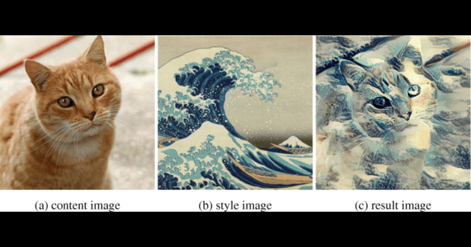
In the process of style transfer, we examine two distinct images: the Style image (shown as 'b' above), which furnishes the desired artistic style, and the Content image (shown as 'a' above), representing the content to be retained in the final stylized image. Utilizing a trained CNN, style transfer identifies the style of one image and the content of another before blending them to produce a third image, referred to as the generated or target image (shown as 'c' above). This resulting image merges the objects and arrangement from the content image with the colors and textures derived from the style image.
The objective of the style transfer technique is to generate a target image (T) where the content closely resembles the content image (C) and the style closely mirrors the style image (S). To assess the content loss during the creation of our target image, we compare its content representation with that of the content image. This process results in what is termed Content loss, quantifying the disparity between the representations of the content image and the target image.
\(Let\)
\(C: \text{Content image} \)
\(T: \text{Target image}\)
\(l: \text{represents a specific layer in the neural network}\)
\(P^l: \text{Content representation at layer } l \text{ for the content image C}\)
\(F^l: \text{Content representation at layer } l \text{ for the target image G}\)
\(L_{\text{content}}: \text{Content loss}\)
$$L_{\text{content}}(C, T, l) = \frac{1}{2} \sum_{i,j}(P_{ij}^l - F_{ij}^l)^2$$
\(P^l_{ij} \) represents the activation of the \(i\text{-th}\) neuron at row \(j\) in layer \(l\) of the pre-trained neural network when the content image \(C\) is passed through it. Essentially, it captures the content information of the content image at that specific layer.
\(F^l_{ij}\) represents the activation of the \(i\text{-th}\) neuron at row \(j\) in layer \(l\) of the same neural network but when the target image \(T\) is passed through it. This captures the feature representation of the target image at that specific layer.
The content loss is calculated by measuring the mean squared difference between the content representation of the content image \((P^l_{ij})\) and the feature representation of the target image \((F^l_{ij})\) at the chosen layer \((l)\). This helps ensure that the target image retains similar content features as the content image at the specified layer. In simpler terms, the content loss guides the optimization process to ensure that the generated image resembles the content of the content image at a specific layer in the neural network.
Now, let's apply the same approach to the style representation of our target image and the style image. The style representation of an image relies on examining correlations among features within individual layers of the network, such as VGG-19. This involves assessing how similar the features within a single layer are, capturing general colors and textures present in that layer.
Typically, we identify similarities across features in multiple layers of the network. By considering correlations across various layers of different sizes, we can establish a multiscale style representation of the input image, encompassing both large and small style features. The style representation is computed as an image passes through the network at the first convolutional layer in all five stacks (in the case of the VGG-19 network). The correlations at each layer are expressed through a Gram matrix.
Suppose you have a set of \(N\) feature maps at a certain layer of a neural network, and each feature map has dimensions \(M\) x \(K\), where \(M\) is the number of spatial positions (pixels) in the feature map, and \(K\) is the number of channels (neurons) in that feature map. You can represent each feature map as a vector by flattening it.
Let \(F\) be the matrix representing these \(N\) feature maps, where each column corresponds to a flattened feature map:
$$F = \begin{bmatrix} \vert & \vert & \dots & \vert \\ F_1 & F_2 & \dots & F_N \\ \vert & \vert & \dots & \vert \end{bmatrix}$$
Here, \(F_i\) is the flattened representation of the \(i\text{-th}\) feature map.
Now, to compute the Gram matrix \(G\), you take the dot product of the transpose of \(F\) with itself:
$$G = F^T . F$$
This results in an \(N\) x \(N\) matrix, where each element \(G_ij\) represents the dot product between the flattened feature map \(Fi\) and \(Fj\). Mathematically, the \(Gij\) element is calculated as:
$$G_{ij} = \sum_{k=1}^{M \times K} F_{ik} \cdot F_{jk}$$
In the context of Neural Style Transfer, the Gram matrix is used to represent the style of an image by capturing these correlations at different layers of the neural network. The style loss is then calculated by comparing the Gram matrices of the style image and the target image, encouraging the target image to have similar style features.
For example, say, we start of with a \(4 \) x \(4\) image, and we convolve it with \(8\) x \(8\) different image filters to create a convolutional layer. This layer will be \(4\) x \(4\) in height and width, and \(8\) in depth. Thinking about the style representation for this layer, we can say that this layer has \(8\) features maps that we want to find the relationship between.
The first step in calculating the Gram matrix, will be to vectorize the values in this layer. The next step is to multiply this matrix by its transpose. Essentially, multiplying the features in each map to get the Gram matrix. Finally, we are left with the square \(8 \) x \(8 \) Gram matrix, whose values indicate the similarities between layers.
Once the Gram matrices for the style image \((A)\) and the target image \((T)\)are computed, the style loss \(L_{style}\) is calculated by comparing these matrices. The style loss at a specific layer \(l\) is computed as the mean squared difference between the corresponding elements of the Gram matrices:
$$L_{\text{style}}(A, T, l) = \frac{1}{4 \times N^2 \times M^2} \sum_{i,j} (T_{ij}^l - A_{ij}^l)^2$$
Here, \(N\) is the number of feature maps, and \(M\) is the number of spatial positions in each feature map.
Now that we have the content loss, which tells us how close the content of our target image is to that of our content image, and the style loss, which tells us how close our target is in style to our style image. We can now add these losses together to get the total loss:
$$L_{\text{total}}(C, S, T) = \alpha \times L_{\text{content}}(C, T) + \beta \times L_{\text{style}}(S, T)$$
\(L_{content} (C, T)\) is the content loss between the content image \(C\) and the target image \(T\)
\(L_{style} (S,T)\) is the total style loss between the style image \(S\) and the target image \(T\)
\(\alpha\) and \(\beta\) are hyperparameters that control the influence of the content and style losses.
In the case of using multiple layers for style representation, the style loss term is often the sum of style losses at different layers:
$$L_{\text{total}}(C, S, T) = \alpha \times L_{\text{content}}(C, T) + \beta \times \sum_{l} \omega_l \times L_{\text{style}}(S, T, l)$$
Here, \(\omega_i\) is a weight associated with each layer.
The full implementation of the Neural style transfer can be found in my github repository