Python for Machine Learning

Introduction

In the previous part of this series, we explored the foundational principles of Python programming essential for comprehending and implementing machine learning algorithms. We covered variables, data types, control statements, and data structures, laying a solid foundation for understanding Python's capabilities in the realm of machine learning.

Building upon that foundation, we now delve into two essential libraries for data manipulation and analysis in Python: NumPy and Pandas.

Introduction to NumPy and Pandas

NumPy, short for Numerical Python, is a fundamental package for numerical computing in Python. It provides support for large, multi-dimensional arrays and matrices, along with a collection of mathematical functions to operate on these arrays efficiently. NumPy is the cornerstone of numerical and scientific computing in Python.

Pandas, on the other hand, is a fast, powerful, and flexible open-source data analysis and manipulation library built on top of NumPy. It offers intuitive data structures, high-performance tools, and data analysis capabilities, making it an indispensable tool for data wrangling and exploration in Python.

In this article, we will explore the core functionalities of NumPy and Pandas, understand how to use them effectively for data manipulation, and delve into some common techniques used in machine learning tasks.

Let's begin by understanding the fundamentals of NumPy and Pandas and how they can be leveraged for machine learning tasks.

Numpy

In the previous lesson, we introduced one of the fundamental data structures in Python, called a List. Lists are commonly used for storing and manipulating data in machine learning tasks. Despite their flexibility in handling different data types, Lists have some drawbacks. They offer limited functionality, occupy significant space in computer memory, and can be time-consuming to process, especially with large datasets. Recognizing these limitations, there arose a need for more efficient data structures, leading to the development of NumPy.

NumPy is a Python library designed to address the shortcomings of Lists. At its core, NumPy utilizes the Array data structure. Unlike Lists, Arrays can only hold one type of data at a time. However, they are significantly more efficient, offering robust functionality while occupying less memory space.

NumPy is a fundamental package for numerical computing in Python, serving as the cornerstone of numerical and scientific computing. Its primary data structure, ndarray, is a powerful N-dimensional array object designed for fast and space-efficient data storage and manipulation.

Key features of NumPy include:

ndarray: A powerful N-dimensional array object providing fast and space-efficient data storage and manipulation.
Mathematical functions: A wide range of functions for performing mathematical, logical, and statistical operations on arrays.
Integration with other languages: NumPy offers tools for integrating C/C++ and Fortran code, making it ideal for numerical computations and data analysis.

For data scientists and machine learning practitioners, NumPy is an essential tool, providing efficient data structures and mathematical functions necessary for data manipulation, preprocessing, and analysis.

Numpy Array Implementation

The following examples demonstrate various methods for creating and manipulating NumPy arrays.

Creating Numpy Array

The most basic form of a NumPy array is a one-dimensional (1-D) array, which can be created using the array() function with a list as its argument.

#import numpy library
import numpy as np

#create a list to use as argument in the array
my_list = [1, 2, 3]

my_array = np.array(my_list)

print(my_array)

#this will print out the list [1, 2, 3]

Another method of creating a NumPy array is by using the arange() function, which is similar to the range() function used for lists. It takes three arguments: the starting value, the end value (one less than the specified value), and the step size for incrementing or decrementing.

#import numpy library
import numpy as np

my_array = np.arange(1, 11, 2)

print(my_array)

#output [1 3 5 7 9]

The linspace() function allows us to create an array with a specified number of elements between a specified range, including both the starting and ending values. This is different from the arange() function mentioned earlier, as linspace() returns an array with a specified number of elements evenly spaced within the specified interval.

#import numpy library
import numpy as np

my_array = np.linspace(1, 100, 5)

print(my_array)

#output [  1.    25.75  50.5   75.25 100.  ]

Creating Numpy Array with fixed item (Element)

Certain problems may necessitate initializing an array with fixed values. NumPy provides special functions to address these requirements, such as zeros(), ones(), and full(). In each case, the argument specifies the size (number of elements) of the array you wish to create.

#import numpy library
import numpy as np

zero_array = np.zeros(5) #array of 5 zeros
print(zero_array)
#output [0. 0. 0. 0. 0.]
one_array = np.ones(5) #array of 5 ones
print(one_array)
#output [1. 1. 1. 1. 1.]
fill_array = np.full(5, 7) #array of 5 7, second arguemet is what to fill
print(fill_array)
#output [7 7 7 7 7]

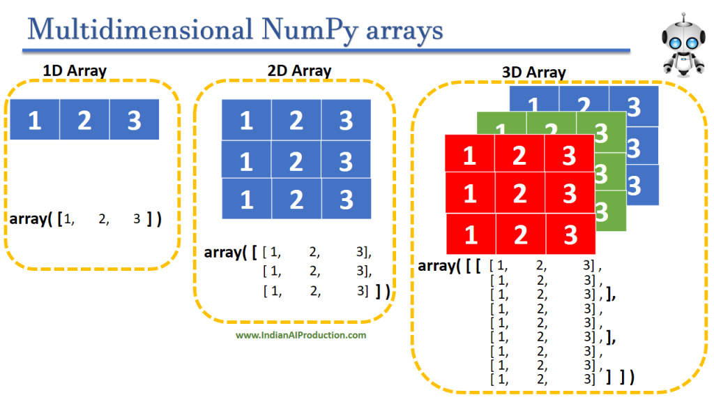
Multidimensional Array

Arrays can also be multidimensional, similar to tables with more than one row and one column. To create a multidimensional array, each row of the array is represented as a list, with each element in the list corresponding to a column. These lists are then separated by commas. The rows and columns must be enclosed in outer square brackets as well.

#import numpy library
import numpy as np

#array with 3 rows 3 columns
multi_dim_array = np.array([[1, 2, 3], [12, 11, 90], [9, 7, 23]])

print(multi_dim_array)

#output [[ 1  2  3]
         #[12 11 90]
         #[ 9   7 23]]

Numpy Array Dimensions

The size function is used to determine the number of elements in an array. The shape function returns the number of rows and columns in an array, while the ndim function is used to find the dimensionality (number of dimensions) of an array.

#import numpy library
import numpy as np

#array with 3 rows 3 columns
multi_dim_array = np.array([[1, 2, 3], [12, 11, 90], [9, 7, 23]])

#number of elements in the array
print(multi_dim_array.size)
#output 9
#number of rows and columns
print(multi_dim_array.shape)
#output (3, 3)
#dimensions of the array
print(multi_dim_array.ndim)
#output 2

Array Math Operation

In this section, you will learn that NumPy allows you to easily perform element-wise addition, subtraction, multiplication, and division on both 1-D and multidimensional arrays. These operations are carried out using the corresponding mathematical symbols: +, -, and *. It's important to note that the behavior of these operations differs from that of Python lists. While adding Python lists would simply concatenate them, resulting in a longer list, attempting to subtract or multiply Python lists would raise an error.

#import numpy library
import numpy as np

arr_1 = np.array([2, 4, 6])
arr_2 = np.array([1, 3, 5])

# Adding two 1-D arrays
addition = arr_1 + arr_2
print(addition)
#output [ 3  7 11]

# Subtracting two 1-D arrays
subtraction = arr_1 - arr_2
print(subtraction)
#output [1 1 1]

# Multiplying two 1-D arrays elementwise
multiplication = arr_1 * arr_2
print(multiplication)
#output [ 2 12 30]

Broadcasting In Numpy Array

Broadcasting in NumPy refers to the ability of NumPy to perform arithmetic operations on arrays of different shapes.

When performing element-wise operations (such as addition, subtraction, multiplication, etc.) on arrays of different shapes, NumPy automatically broadcasts the arrays to have compatible shapes. This allows the operations to be performed element-wise without requiring the arrays to have the same shape.

For example, if you have a 1D array of shape (3,) and you want to add a scalar value to it, NumPy will automatically broadcast the scalar value to have the same shape as the array (3,), and then perform the addition operation element-wise.

vector = np.array([1, 2])
vector * 1.6

#output array([1.6, 3.2])

Pandas

Pandas is a fast, powerful, and flexible open-source data analysis and manipulation library built on top of NumPy. It provides easy-to-use data structures and data analysis tools for Python programming, making it an essential tool for data wrangling and exploration.

Key features of pandas include:

DataFrame: A two-dimensional, size-mutable, and heterogeneous tabular data structure with labeled axes (rows and columns). DataFrame is ideal for working with structured data.
Series: A one-dimensional labeled array capable of holding data of any type, including integers, floats, strings, and Python objects.
Data manipulation tools: A wide range of functions and methods for indexing, slicing, merging, reshaping, and aggregating data.
Data reading and writing: Tools for reading and writing data from and to various file formats, including CSV, Excel, SQL databases, and JSON.

Pandas is widely used for data analysis, data preprocessing, and data visualization tasks in Python, making it an indispensable tool for data scientists, analysts, and machine learning practitioners.

Pandas Implementation

The examples below illustrate different methods for creating and manipulating both one-dimensional pandas Series and two-dimensional pandas DataFrames.

Creating Series

A Series is an enhanced one-dimensional array. It goes beyond supporting zero-based indices; it also allows for custom indexing, including non-integer indices such as strings.

#import pandas
import pandas as pd

#create a pandas series from list
grades = pd.Series([23, 100, 30])

print(grades)
#output 0     23
        #1    100
        #2     30
        #dtype: int64

The Series provides many methods for common descriptive statistical tasks, including count, mean, min, max, std (standard deviation), and more.

#import pandas
import pandas as pd

#create a pandas series from list
grades = pd.Series([23, 100, 30])

print(grades.count())
#output 3
print(grades.mean())
#output 51.0
print(grades.min())
#output 23
print(grades.max())
#output 100
print(f'{grades.std():.2f}')
#output 42.58

Creating Dataframes

A DataFrame is an enhanced two-dimensional array. Like Series, DataFrames can have custom row and column indices, along with additional operations and capabilities that make them more convenient for many data science-related tasks.

#import pandas
import pandas as pd
#given dictionary
grades_dict = {
        'wally': [78, 19, 100],
        'tayo': [89, 48, 90],
        'sam': [70, 17, 29],
        'bola': [90, 86, 100]
}

#create a pandas table using the dictionary 
grades = pd.DataFrame(grades_dict)

print(grades)

#output
#         wally  tayo  sam  bola
#    0     78    89   70    90
#    1     19    48   17    86
#    2     100    90   29   100

In Pandas, you can access each column by specifying the column name inside square brackets after the DataFrame name, as shown below.

#import pandas
import pandas as pd
#given dictionary
grades_dict = {
        'wally': [78, 19, 100],
        'tayo': [89, 48, 90],
        'sam': [70, 17, 29],
        'bola': [90, 86, 100]
}

#create a pandas table using the dictionary 
grades = pd.DataFrame(grades_dict)

#accessing a particular column
print(grades['wally'])

#output
#         wally  
#    0     78    
#    1     19    
#    2     100
#    Name: wally, dtype: int64

According to the Pandas documentation, accessing DataFrame items with [] is not the most optimized approach, as it creates a copy of the data. This can lead to logical errors if you attempt to assign new values to the DataFrame. Therefore, it is highly recommended to use the loc and iloc attributes for accessing items in a DataFrame.

You can access a row by its row name (if it has a string row name) using the loc attribute and by its index (integer starting from 0) using the iloc attribute.

#import pandas
import pandas as pd
#given dictionary
grades_dict = {
        'wally': [78, 19, 100],
        'tayo': [89, 48, 90],
        'sam': [70, 17, 29],
        'bola': [90, 86, 100]
}

#create a pandas table using the dictionary 
grades = pd.DataFrame(grades_dict)

#accessing a row 0
print(grades.iloc[0])

#output
#wally    78
#tayo     89
#sam      70
#bola     90
#Name: 0, dtype: int64

Slicing can be used to obtain a portion of the table. Some of these are implemented below.

#import pandas
import pandas as pd
#given dictionary
grades_dict = {
        'wally': [78, 19, 100],
        'tayo': [89, 48, 90],
        'sam': [70, 17, 29],
        'bola': [90, 86, 100]
}

#create a pandas table using the dictionary 
grades = pd.DataFrame(grades_dict)

#slicing from the first row(row 0) to the second row (row 1) 
print(grades.iloc[0:2]) # this is used to get consecutive rows

#output
#      wally  tayo  sam  bola
#0     78    89   70    90
#1     19    48   17    86

#import pandas
import pandas as pd
#given dictionary
grades_dict = {
        'wally': [78, 19, 100],
        'tayo': [89, 48, 90],
        'sam': [70, 17, 29],
        'bola': [90, 86, 100]
}

#create a pandas table using the dictionary 
grades = pd.DataFrame(grades_dict)

#getting the first column (column 0) and second column (column 2) 
print(grades.iloc[[0, 2]]) # this is used to get non-consecutive column

#output
#    wally  tayo  sam  bola
#0     78    89   70    90
#2    100    90   29   100

#import pandas
import pandas as pd
#given dictionary
grades_dict = {
        'wally': [78, 19, 100],
        'tayo': [89, 48, 90],
        'sam': [70, 17, 29],
        'bola': [90, 86, 100]
}

#create a pandas table using the dictionary 
grades = pd.DataFrame(grades_dict)

#get the first two consecutive rows, with its 
#first two consecutive column
#it takes last index-1 (as in 2-1 = 1 as the upper bound)
print(grades.iloc[0:2, :2]) 


#output
#  wally  tayo
#0     78    89
#1     19    48

Finally, you can obtain a quick summary of its main descriptive statistics using the describe() function, as shown below:

This concludes the final part of the Python for Machine learning course, and it is our hope that you will actively engage with the material by practicing with the provided code snippets. Furthermore, to reinforce your understanding of these concepts, I have prepared a complementary GitHub repository where you can find additional practice questions along with their respective solutions in case you encounter difficulties.

Feel free to explore, contribute, and share the repository with your peers. Your continuous support is greatly appreciated!

Remember to Follow, Like, Share, and Subscribe for future updates. Until next time, happy coding!

aljebra school